Over the summer, Social Innovation Simulation will be posting a series of technical tutorials designed to acquaint those interested with some of the technologies we’re working with.

This tutorial describes how you can implement a system of ordinary differential equations in Java and use them in a project.

Estimated Time: 1–2 hours

Dependencies: basic Java knowledge, basic Eclipse knowledge, knowledge of differential equations

What are Differential Equations and Why Are They Useful?

Differential equations are simply equations that show a relationship between a set of variables and their derivatives. Something as simple as:

dx/dt = 5x

is a differential equation, however differential equations can get much more complicated than that. Differential equations are used in a number of different areas, including population growth, the modelling of weather patterns, and the calculation of investment returns.

Since there are so many potential applications for differential equations, it is very useful to be able to implement them in software programs. Writing such programs can help those that use these equations on a day-to-day basis. The following tutorial will explain how to implement and use a set of differential equations in Java. This will enable you to write programs using differential equations for any number of different fields in which you have the necessary background.

Tutorial – Differential Equations

Import the library that contains the functions you need. These are fairly basic instructions on importing any library into a Java project while you are using Eclipse. If you have done this before then all you need to do is import the Apache Commons math library (which can be found here or in the Resources section). If you have already imported the Apache Commons math library, then skip to step 2.The first step for importing the Apache Commons math library is to download the latest version from the Apache Commons website: http://commons.apache.org/proper/commons-math/download_math.cgi.
Unless you have a reason for needing the source code, it is best to just download the binaries, since you don’t have to do anything to them to use them. Once you download the binaries, it is also best to create a new folder for your Java libraries so that they are easier to find. You can put your new binaries in it. There are many useful libraries out there that you should check out. You should have a place to put them all! 🙂

Next, open the project in Eclipse that you want to include the libraries in. Once you’ve opened the project in Eclipse, copy all the files from the zip file you downloaded, and paste them into the “lib” folder of your project.

lib folder

Finally you need to include these libraries in your project classpath. This is very important since you will get errors in your project if you do not include the external libraries in your classpath. To do this, right-click on your project in the navigation window on the left, and click on “Preferences”. Then navigate to “Java Class Path” and click “Add JARs…”. Once this window opens up, navigate to the “lib” folder of your project and select all the files that you just copied over. Then click “OK” and “OK” again. Now you’re all ready to use your new library!

Click OK

Click OK
Find the differential equations you want to model. In order to model a set of differential equations we first need to have some! For this tutorial we will be using the Lorenz Equations since they are well known, and aren’t very complicated. More information about the Lorenz Equations can be found here, but you can use any set of ordinary differential equations you want. The Lorenz Equations consist of 3 equations in 3 variables (x, y and z) with 3 constants (which we will call A, B and C) — all of which are related to time. The equations are as follows:
```
dx/dt = A(y - x)
dy/dt = x(B - z) - y
dz/dt = xy - Cz
```
Implement the differential equation class that our imported library gives us. We are going to implement the FirstOrderDifferentialEquations class for this example. The first step is to create the class that is implementing our imported class, which we are going to call LorenzODE. To create this class simply click the green circle with a C inside in the top-left corner. Then enter the name of your class (in this case “LorenzODE”) and the package your class will be put in (for simplicity we are using “lorenzODE”). This will create our class declaration. We need to change our class declaration a little bit to implement our imported class as follows:
public class LorenzODE implements FirstOrderDifferentialEquations{ }

You’ll probably notice that this gives you an error. This is just because we haven’t imported our math library into this file yet. This can easily be fixed by hovering over the word underlined in red (which should be FirstOrderDifferentialEquations), and then, when the error-message-tooltip pops up, click on ‘Import FirstOrderDifferentialEquations’. Our class file will now look like this:
package lorenzODE;

import org.apache.commons.math3.ode.FirstOrderDifferentialEquations;

public class LorenzODE implements FirstOrderDifferentialEquations{
}

You will probably still see an error in this class because the abstract functions from the FirstOrderDifferentialEquations class have not been implemented yet. We will fix this later on.
Add functionality to your new class. Now we are going to actually add in the logic for our class. If you look back at the Lorenz Equations that we’re using, you’ll notice we have 3 constant values that we need to track (which we named A, B and C). So we need 3 private doubles for our constant values:
public class LorenzODE implements FirstOrderDifferentialEquations{ private double A; private double B; private double C; }Next we are going to create the constructors for our class. Firstly we want a constructor that takes 3 doubles as arguments, one for each constant. This one is pretty straightforward:
public LorenzODE(double A, double B, double C){ this.A = A; this.B = B; this.C = C; }

We also want to create a default constructor (so that we don’t always need to specify our constants). The defaults we are going to use for the Lorenz Equations are A = 10, B = 28 and C = 8/3 (these were the original values that Lorenz used when studying this system of equations):

public LorenzODE(){ this.A = 10; this.B = 28; this.C = 8/3; }

Now that we’ve created the constructors, we need to implement two more functions. The first function is called getDimension(). This function (as you would expect) returns the dimension of the differential equation. The dimension is of the differential equations is the number of variables in the system of equations (in this case 3):
public int getDimension(){ return 3; }

Finally, we need to implement the actual equations. In this step (shown below) we implement the function computeDerivatives() which returns void and takes in 3 arguments: a double representing the current time, an array of doubles representing the current values of the 3 variables, and another array of doubles representing the current values of the derivatives of the 3 variables.

We then implement the 3 equations of the Lorenz Equations.

Putting everything together we get the following:
public void computeDerivatives(double t, double[] xyz, double[] xyzDot){ xyzDot[0] = A * (xyz[1] - xyz[0]); xyzDot[1] = xyz[0] * (B - xyz[2]) - xyz[1]; xyzDot[2] = (xyz[0] * xyz[1]) - (C * xyz[2]); }

If you notice in the code above the first element of the array “xyz” is the x variable, the second is the y variable and the third is the z variable. Similarly the first element of the array “xyzDot” is the derivative of the x variable, and so on.

After all of that, our class has been implemented and looks like this:
public class LorenzODE implements FirstOrderDifferentialEquations{ private double A; private double B; private double C;public LorenzODE(double A, double B, double C){ this.A = A; this.B = B; this.C = C; }public LorenzODE(){ A = 10; B = 28; C = 8/3; }public int getDimension(){ return 3; }public void computeDerivatives(double t, double[] xyz, double[] xyzDot){ xyzDot[0] = A * (xyz[1] - xyz[0]); xyzDot[1] = xyz[0] * (B - xyz[2]) - xyz[1]; xyzDot[2] = (xyz[0] * xyz[1]) - (C * xyz[2]); } }
Using the system of equations.
Now that we have our system of equations set up, we want to actually use it. For this example, we are going to set up a new class to run a “main” function. This will show how you would use the differential equations we have specified above. When you use your own differential equations, you will just add the functionality into whatever class you need it in.To set up, we create a new class just like before. We will call that new class “temp.” (look back at step 3 to see how to do this). We need to import a few classes from the Commons Math library so after everything is set up it should look like this:
package lorenzODE;import org.apache.commons.math3.ode.FirstOrderDifferentialEquations; import org.apache.commons.math3.ode.FirstOrderIntegrator; import org.apache.commons.math3.ode.nonstiff.DormandPrince853Integrator;public class temp { public static void main(String[] args){} }

These imports will make more sense once we’ve finished writing our main function, but for now it’s easiest just to import them to avoid error messages. The first step in using our code is to choose an integrator to use. We are going to use the Dormand-Prince 8(5,3) integrator that the math library provides, but you can use any of the other integrators found in the math library (a list of the integrators can be found here, if you skip down to section 13.4 (Available Integrators)). The integrators in that list simply vary in the way that they calculate the variable values and derivatives at each time step, but all should work for this example if you want to try out other types of integrators.

Since we are using the Dormand-Prince 8(5,3) integrator, we first need to create a new instance of this integrator. The constructor for this integrator (along with most of the Adaptive Step integrators found in the link above) takes in 4 doubles: one for the minimum step the integrator can take, one for the maximum step, one for the allowed absolute error, and one for the allowed relative error. Most of these won’t matter very much (unless you know that you need a certain amount of certainty) as long as all the numbers (except the 2nd) are fairly small. For this example we’ll use the following:

FirstOrderIntegrator dp853 = new DormandPrince853Integrator(1.0e-8, 100.0, 1.0e-10, 1.0e-10);

We also have to create a new instance of our class implementing the Lorenz Equations:

FirstOrderDifferentialEquations ode = new LorenzODE();

Finally we need to create an array of doubles with the starting values for all of our variables. For all three, we are just going to default these starting values to 1.0:

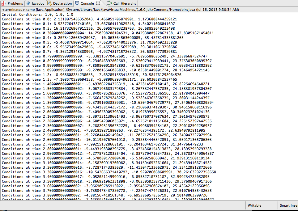
double[] xyz = new double[] { 1.0, 1.0, 1.0 };

Now we are all set up to actually use our differential equations (finally! :). The function that we want for this is the integrate() function from our integrator. This function takes in 5 arguments: the implementation of the FirstOrderDifferentialEquations class, the starting time of our integration, an array with the starting values for our differential equations, the ending time of our integration, and the array that the starting values for our differential equations should be recorded in. For this example we are simply going to print out the values for 200 time steps of 0.1 to show that you can access these values.

Conveniently we’ve already set up the implementation of the FirstOrderDifferentialEquations class (our “ode” variable). We are also going to use the same array that has the starting values for the equation variables to store the ending values of the variables to make it much easier to loop through the differential equations. All we need to do now is set up a for-loop, which can be done as follows:

for(double i = 0.0; i < 20; i += 0.1){ dp853.integrate(ode, i, xyz, i + 0.1, xyz); System.out.println("Conditions at time " + i + ": " + xyz[0] + ", " + xyz[1] + ", " + xyz[2]); }

This loop will simply modify the variable values for each step of 0.1 and then print out the current time and the values of the variables at this time. Now that our main class is finished, we just need to run the project. Simply go to the “Run” menu, mouse-over “Run As” and click “Java Application”. You should see something like this in your output:

Output

And now you’re done! As you can see, once you have this math library imported, it is very easy to implement and use any differential equation that you want.

Deliberate Practice

Now that we’ve gone over how to implement and use a differential equation, the next step is to actually integrate this into a real project. If you have a project that you are working on that needs to use differential equations, then you can use that to practice.

If not, think of a simple project that would be able to use a differential equation, and try implementing what you learned above. Here’s a list of some examples that you can try:

Implement a weather system that uses a differential equation to get: the temperature, the wind speed, and the humidity
Implement a model of moving objects that get their positions from a differential equation (can use the same differential equation for all of them or different ones for each object)
Generate a “picture” using blocks of colour where each block of colour is determined by a different step in a differential equation (using a numerical scale to correspond to different colours – you can use a red-green-blue colour scale if your differential equation has 3 variables)

Remember, you don’t have to use these examples. The point is to take what you learned in the tutorial and implement it in a program that does more than just print values.

I hope this tutorial helped you learn more about differential equations, and how you can use them in Java! If you are looking for more information on this topic, check out the resources section below.

Resources

Here is a list of some of the better resources to get more information about differential equations, and how to implement them in Java using the Apache Common math library.

Apache Commons resource:
http://commons.apache.org/proper/commons-math/userguide/ode.html

More information on differential equations:
http://tutorial.math.lamar.edu/Classes/DE/DE.aspx
http://www.sosmath.com/diffeq/diffeq.html

Apache Commons API:
http://commons.apache.org/proper/commons-math/apidocs/index.html