Over the summer, Social Innovation Simulation will be posting a series of technical tutorials designed to acquaint those interested with some of the technologies we’re working with.
This tutorial describes how you can use a JavaScript language called D3 (“data driven documents”) to do visualizations with maps.
Estimated Time: 1 – 2 hours
Dependencies: Basic HTML, basic D3, setting up a server.
Tutorial – Making Maps on D3

Level 1: Creating a Basic Map using TopoJSON
-
Set up a local server in your workspace directory.
e.g.,
Once the server is running, you can access files in your workspace directory from a web browser like Chrome. Simply type “localhost:8080” into your browser’s address bar. Accessing specific html pages requires us to add “/filename.html” to the end of the address, e.g., http://localhost:8000/filename.html
Because we will be linking json files from our computer to our html page, some browsers will not load our page for security reasons.
-
Acquire a nice and organized TopoJSON file. For this tutorial we will be using data kindly provided to us by Mike Bostock on GitHub since it has data on US counties as well as its states:
https://raw.github.com/mbostock/topojson/master/examples/us-10m.jsonCopy and paste the code into a plain text editor (e.g., TextWrangler on Mac or Notepad++ on PC) and save as “us-topo.json”.
-
Set up your HTML framework and import the D3 and TopoJSON library:
<script src= "http://d3js.org/d3.v3.min.js"></script>

<script src= "http://d3js.org/topojson.v1.min.js"></script>

You can also use the HTML template below:

<!DOCTYPE html>

<html>

<head>

<meta charset="utf-8">

<script src="http://d3js.org/d3.v3.min.js"></script>

<script src="http://d3js.org/topojson.v1.min.js"></script>

<style></style>

</head>

<body>

<script type="text/JavaScript">
/* D3 code here */</script>
</body>
</html> -
Create an SVG element within the
<script></script>tags where the/* D3 code here */comment is found. We will be building our map within the SVG canvas, and so we set the width and height to 1000 and 500 respectively.Important note: At this point, it will not display anything.
var w = 1000;

var h = 500;

var svg = d3.select("body").append("svg")

attr("width", w)

.attr("height", h);-
To make sure you have done this correctly (and are using a Chrome browser), right click in your browser window, click “Inspect Element” and verify that you have indeed created created an svg element within the body of your html code. It should look something like this:
-
-
Specify a projection1 and a path generator.
var projection = d3.geo.albersUsa()

var path = d3.geo.path()

.projection(projection);-
d3.geo.path()is our path generator, and will create a path based on a bounded geometry object2, which contains the coordinates of the boundaries for each state/county. -
By default,
d3.geo.path()uses the albersUsa projection, so “.projection(projection)” is not necessary. However, you can change “d3.geo.albersUsa()” to any of the common map projections listed here: https://github.com/mbostock/d3/wiki/Geo-Projections-
Note that if you choose a different projection, you may have to tweak, as some of these projections are made for world maps.
-
You can also write your own projection function!
-
-
-
Add code to look inside your us-topo.json file. As you’ve probably noticed, our json file is lengthy, convoluted, and written all in one line. To get a sense of the hierarchy of the data, we can look inside the console again for a more organized arrangement of the json file. To do this, we need to add this to our html file, beneath our svg element:
d3.json("us-topo.json", function(us) {
console.log(us);
});-
Observe that the parameter within the function is the name we will be using throughout the d3.json() code to refer to our data.
-
Inside the console you will find information about counties, their boundary coordinates (which are listed as arcs in TopoJSON files) and their geometry type (Polygon, Multipolygon, etc), an interesting read!
If this is running correctly, you should see this at the bottom or side of your browser:
-


(nb. no map in sight yet!)

-
Bind geometry objects to paths. In order to use our path variable, we will need to convert our TopoJSON file back to GeoJSON using topojson.feature(). When working with a GeoJSON file (like in your deliberate practice), all you need is .data(us.features)
svg.selectAll(“append”)
.data(topojson.feature(us, us.objects.counties).features)
.enter()
.append(“path”)
.attr(“d”, path);-
SVG paths are defined by one attribute, “d”, which dictates how we want to draw a line from one point in our data to another, essentially how we want to shape our data, using a series of commands. Our “path” variable simplifies things for us. The path variable determines the shape of our data based on the type of geometry object it is (see GeoJSON Objects below). For more information on paths check out: https://developer.mozilla.org/en-US/docs/SVG/Tutorial/Paths
-
After peeking at the hierarchy of your json file in the console, you can see how this code is accessing the data.
-
Don’t care for counties? Maybe you prefer states. DIY!
-
Your final product should look like either of these:
-

Deliberate Practice
Try creating a basic map using the GeoJSON code for Canada found here:
https://raw.github.com/mdgnkm/SIG-Map/master/canada.json
You can use the following code for the dimensions of the svg canvas and the projection:
-
svg dimensions:
var w = 800; var h = 600; -
projection:
var projection = d3.geo.azimuthalEqualArea()
.rotate([100, -45])
.center([5, 20])
.scale(800)
.translate([w/2, h/2])
When you get this working, you should see the whole map:

Level 2: Styling Your Map
-
Colours
-
Choosing colours
-
We can choose each colour we want to use by defining a “function” or scale that takes in our data and returns a colour assignment. For example, colouring the map of USA, we can take all the state ids (found in the json file) as our domain, and define each colour as the range:
var colour = d3.scale.linear()
.domain([0, 52])
.range(["rgb(217,95,14)","rgb(254,196,79)",
"rgb(255,247,188)"]);-
Note that we defined RGB values to pick our colour. We can also use HEX values and simple colour names like “red”, “green”, “violet”. A great colour reference for representing sequential, diverging, or qualitative data using RGB values is: http://colorbrewer2.org/
-
-
We can also use built-in colour scales in D3:
var colour = d3.scale.category20c(); -
Here are a few more colour categories:
https://github.com/mbostock/d3/wiki/Ordinal-Scales#categorical-colors
-
-
Applying colours
-
After our chain of code from Step 7, we can add an attribute to change the fill of each object:
.attr("fill", function(d, i) { return colour(i); }); -
OR we can assign classes to objects and then change them using CSS:
D3 – .attr("class",function(d,i) { return "state" + I; });
CSS – …
.state19 { fill: #222; }
.state20 { fill: #aaa; }
…-
This is rather inefficient for our purposes, but if we wanted to use the same colour for certain states that fall into a particular statistical class/range, this would be the way to do it!
-
-
-
-
Borders
-
Can be made via D3 or CSS by assigning classes for each state:
-
D3 – .attr(“stroke”, “#fff”)
-
CSS – .state-border { stroke: #000″; }
-
-
OR we can mesh together all the boundaries for each state using topojson.mesh:
svg.append("path")
.datum(topojson.mesh(us, us.objects.states,
function(a, b) { return a !== b; }))
.attr("stroke", "#fff")
.attr("d", path);-
The function prevents us from creating double strokes for overlapping borders
-
-
Other useful attributes include:
-
stroke-linejoin: determines the shape of the edges of borders – round, line, miter: https://developer.mozilla.org/en-US/docs/SVG/Attribute/stroke-linejoin -
stroke-dasharray: creates a dashed border and controls the pattern of dash and gap lengths – num, num: https://developer.mozilla.org/en-US/docs/SVG/Attribute/stroke-dasharray -
stroke-width: by default it is set to 1px
-
-
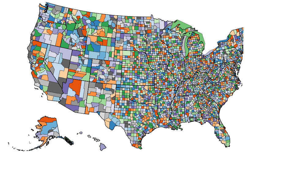
Here is an example of a US county map created by Nathan that is styled with solid borders for states and dashed borders for counties, and is coloured to the extreme:
-
Level 3: Integrating Statistical Information
For this exercise, let us use the canada.json and immigration.csv file found here:
https://github.com/mdgnkm/SIG-Map
Hopefully you’ve done the first deliberate pracitice. If not, it’s not too late!
-
Acquire a tsv/csv file whose data corresponds with those in a separate Topo/GeoJSON file.
-
Use a text editor to peer into canada.json and immigration.csv. Tweak any province name discrepancies between the two files, if they exist (i.e. check that the names of each province/territory is spelt the same in both files).
-
-
Include the Queue.js library in your HTML document.
<script src="http://d3js.org/queue.v1.min.js"></script>-
Queue.js will allow us to load both our json and tsv/csv data before manipulating them.
-
-
Define your classes using the d3 quantize scale function. Set the domain boundaries to:
var quantize = d3.scale.quantize()
.domain([0, 102000])
.range(d3.range(3).map(function(d,i) {return "class"+i;}));-
This takes in the total number of immigrants in each province, ranging from 9 to 102,00, and returns “classi” where i is the index of an array of length 3, created by
d3.range(3). -
We could also write:
.range([“class0”, “class1”, “class2”])
especially since there are so few data classes. For the US choropleth exercise below, the previous range definition is much better to work with, especially since we have many more data classes and wouldn’t want to manually type them out. -
Perhaps now is the time you would also like to define the fill colour of each class within the
<style></style>tags. Refer to Applying Colours Part ii in the section above and use http://colorbrewer2.org/ to choose your colours. Our classes should be class0, class1 and class2:.class0 { fill: rgb(254, 224, 210); }
.class1 { fill: rgb(252, 146, 114); }
.class2 { fill: rgb(222, 45, 38); }
-
-
Create a new dictionary that will later associate province names (key) with their immigration total (value):
var immByProv = d3.map();-
We will use this dictionary to access the csv file data using json data properties (i.e. the names of the provinces found in canada.json)
-
-
Use Queue.js to load your json and csv files. You can remove the d3.json code in your html from the previous exercise as we will be using a different function (myFunction) to create the body of the map.
queue()
.defer(d3.json, "canada.json")
.defer(d3.csv, "immigration.csv", function(d)
{ immByProv.set(d.Geography, +d.Total); })
.await(myFunction);
This will load any files before running the function within .await(). Within the second .defer(), we added an extra parameter to fill our dictionary with province names and their corresponding immigration total. This is why it is important to verify that both files have the same province names! -
Define myFunction to bind provinces to a path and assign classes based on the immigration totals:
function myFunction(error, can) {
svg.append("g")
.attr("class", "provinces")
.selectAll("path")
.data(can.features)
.enter()
.append("path")
.attr("class", function(d) { return quantize(immByProv.get(d.properties.NAME)); })
.attr("d", path);
};-
immByProv.get() returns the value associated with each province name in our dictionary.
-
-
Style it! We already have defined styles for each class from step 3c, so now all we need to add is the style for provinces to create distinct borders. We add this to the <style></style> tags:
.provinces {
stroke: #000;
stroke-linejoin: round;
}
And voila! You have just created a choropleth map based on total immigrants per province.
More Deliberate Practice
Use your map of USA from Level 1 of the tutorial along with the unemployment.tsv file (found here: https://gist.github.com/mbostock/4060606#file-unemployment-tsv) to create another choropleth map. If you are stuck, you can take a peek at Mike Bostock’s choropleth map, which uses the same files (and pretty much the same code): http://bl.ocks.org/mbostock/4060606
Appendix
Map Projections1
A map will have some sort of distortion one way or another, but depending on its purpose, it will try to preserve one of the following:
-
Equivalence/Equal Area (area):
-
Accurately represents area size proportional to ground area
-
Used when measurements are important, when angles/shape can be forgone
-
e.g. Azimuthal Equal Area
-
-
Equidistance (scale/distance)
-
Correctly represents distances from one point to another BUT only in certain directions (meridian/parallel lines)
-
e.g. Conic Equidistant
-
-
Conformity (angles/shape)
-
Angles and shapes are represented accurately, scale is the same in any direction
-
Used for navigation and to make the Northern Hemisphere/Antarctic look larger than they are (which makes Australia very bitter)
-
e.g. Mercator
-
-
Note: conformity and equivalence are mutually exclusive
-
Another note: There are some projections that preserve none of these, but instead make a compromise and distort very little of each. A famous example of this is the Robinson projection, which is commonly used for world maps.
-
More information on D3 projection centers, rotations, scales, etc:
http://www.d3noob.org/2013/03/a-simple-d3js-map-explained.html
GeoJSON Objects2
A GeoJSON object is either a geometry object, containing coordinates to indicate a shape, or a feature object which includes a section for geometry objects (“geometry”) and a section for their properties (“properties”). It can also be a FeatureCollection or GeometryCollection, which must contain a section for geometry objects (“geometries”) and a section for feature objects (“features”), respectively.
Notes:
- If you console.log the us-geo.json file, you will see the object containing all data on the US states has “FeaturesCollection” as its type, literally meaning a collection of feature objects. Within each object in “features” is a section for geometry and properties. Note that the type of each object is “Feature”, and within their geometry there is an indication of which type of geometry object it is (e.g., Polygon, Line, MultiPolygon, Point).
- For a list of types of geometry objects and more info on GeoJSON objects here is the official GeoJSON link: http://www.geojson.org/geojson-spec.html#geojson-objects
- See this excellent tutorial on basic maps. This will also tell you how to find your own data (often as a shapefile (.shp) and how to convert it using ogr2ogr and GDAL): http://bost.ocks.org/mike/map/
